Validation • OECDsppps

library(dplyr)
library(tidyr)
library(gt)
library(ggplot2)
library(OECDsppps)

Overview

Data validation is carried out to confirm the validity of price statistics at various levels of aggregation, from the initial item-level price quotes to the basic heading level and upwards, as well as comparing household expenditure weights across regions. The process aligns with current recommendations; see ICP (2021), World Bank (2013) and European Union/OECD (2024) for more information.

The validation steps are:

Intra-regional validation analyses individual and aggregate price quotes within the same region and across regions of the same country
Inter-regional validation performs prices validation across all regions and countries, ensuring that average prices are based on comparable products in regions across countries and that products have been accurately priced.
Validation of alternative data sources describes the validation process of alternative data sources
Validation at basic-heading level covers the validation of price indices at the basing-heading level
Expenditure weights validation describes the validation of household consumption expenditure
Validation beyond basic-heading level concerns the validation of price indices beyond the basing-heading level

Data used in this vignette is taken from official UK microdata from the United Kingdom Office for National Statistics (ONS). Similar data was recently used in Hearne and Bailey (2025) and is publicly available:

uk_cpi() is a snipped of the UK CPI microdata containing two products: White sliced loaf branded 750 grams (COICOP 1010103) and carpenter hourly rate (COICOP 410518).

head(uk_cpi, n = 3) |>
  group_by(Year, coicop_5d, `Product code`, `Product description`) |>
  gt()

Date of quote	Reference quantity	Unit of reference quantity	Region	Shop identifier	Type of shop	Quantity observed	Unit of observed quantity	Price observed	Reference quantity price
2018 - 01.1.1.3 - 210111 - WHITE SLICED LOAF BRANDED 750G
201801	750	1	South East	1	Multiple	750	1	1.00	1.00
201801	750	1	South East	1	Multiple	750	1	1.00	1.00
201801	750	1	North West	1	Multiple	750	1	1.45	1.45

1 Intra-regional validation

Intra-region validation establishes that price collectors within the same region and across regions of the same country have priced products that match the product specifications and that the prices they have reported are correct. This is done in two stages, which correspond to the outlier detection of (a) individual prices and (b) average price aggregates.

1.1 Individual price outlier statistics

For each product, a Price Observation Table is obtained, containing a characterisation of the individual product as well as two individual price outlier statistics, the ratio-to-average price test and the t-value test; see World Bank (2013), table 9.1a for an extensive example.

Ratio-to-average price test: The ratio of an individual price observation \(i\), \(P_{i}\), of a specific product \(j\) and the observed average price for the product, \(\mu_j\). An observed price passes the this test if the ratio is between 0.5 and 1.5. This simple check flags potential outlier values values without relying on standard deviation, which can itself be distorted by outliers (World Bank 2013, 251).

\[ ratio-to-average = p_{ij}/\mu_j \]

T-value test: The ratio of the deviation of an individual price observation from the average reference quantity price for the product and the standard deviation of the product. To pass the test, the ratio must be 2.0 or less in absolute terms; any value greater than 2.0 is suspect because it falls outside the 95 percent confidence interval.

\[ t-val = (p_{ij} - \mu_{P_j}) / \sigma_{P_j} \]

Individual price quotes that do not pass these tests are flagged in the Price Observation Table. The price observation table is generated with the function valid_pot().

Example using UK CPI microdata

# Price Observation Table  ---------
uk_pot <- uk_cpi |>
  select(Year, `Product code`, , `Product description`, `Reference quantity price`) |>
  group_by(Year, `Product code`, `Product description`) |>
  valid_pot(price_quote = "Reference quantity price") |>
  ungroup()

head(uk_pot, n = 3) |>
  gt() |>
  tab_header(
    title = md("**Price Observation Table**"),
    subtitle = md("Example for `item_id` = 210111")
  ) |>
  fmt_number(
    columns = c(
      `Ratio-to-average price test`,
      `T-value test`
    ),
    decimals = 2
  )

Year	Product code	Product description	Reference quantity price	Ratio-to-average price test	T-value test	Ratio-to-average price test FLAG	T-value test FLAG
Price Observation Table
Example for `item_id` = 210111
2018	210111	WHITE SLICED LOAF BRANDED 750G	1.00	0.96	−0.21	FALSE	FALSE
2018	210111	WHITE SLICED LOAF BRANDED 750G	1.00	0.96	−0.21	FALSE	FALSE
2018	210111	WHITE SLICED LOAF BRANDED 750G	1.45	1.39	1.83	FALSE	FALSE

# Visualisation of price distribution ---------
uk_pot |>
  select(
    `Product code`,
    `Ratio-to-average price test`:`T-value test`
  ) |>
  pivot_longer(`Ratio-to-average price test`:`T-value test`) |>
  mutate(
    is.outlier = case_when(name == "Ratio-to-average price test" & (value < 0.5 | value > 1.5) ~ "Test not passed",
      name == "T-value test" & ((value > 2) | (value < -2)) ~ "Test not passed",
      .default = "Test passed"
    ),
    is.outlier = factor(is.outlier, levels = c("Test passed", "Test not passed"))
  ) |>
  ggplot(aes(x = value, fill = is.outlier)) +
  facet_wrap(~name, scales = "free") +
  geom_histogram(bins = 30) +
  labs(
    title = "Individual price outlier statistcs",
    subtitle = "White sliced loaf branded 750G, 2018",
    x = "",
    fill = ""
  ) +
  theme_minimal() +
  theme(legend.position = "top") +
  scale_fill_manual(values = c("#a3bbdd", "#2a4691"))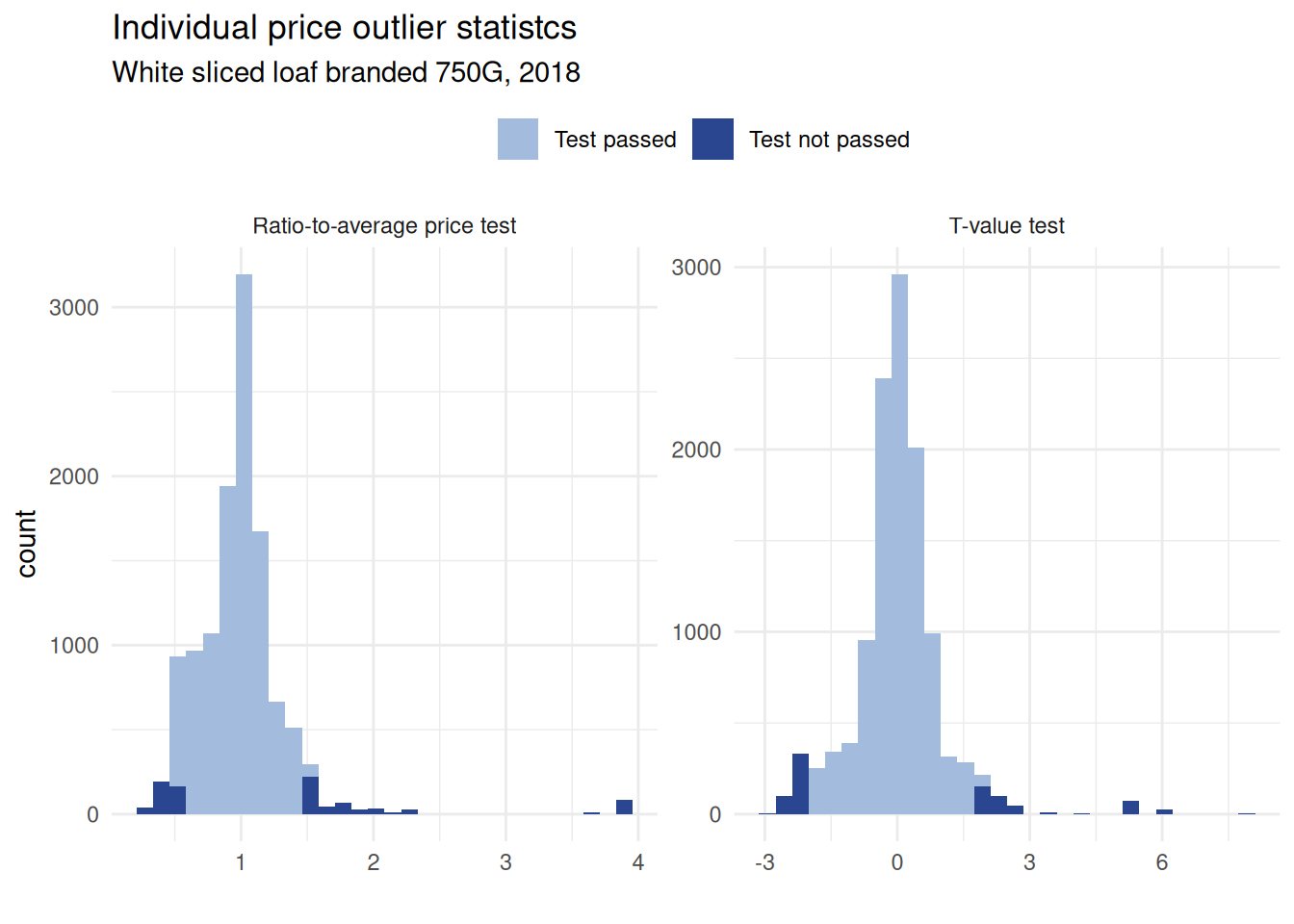

1.2 Aggregate price statistics

This stage involves identifying extreme values among the average prices of the products listed in the Average Price Table. An extreme value is defined as an individual price or average price that for a given test scores a value that falls outside a predetermined critical value and is build on two average price outlier statistics, which are summarised in the Average Price table; see World Bank (2013), table 9.2a and 9.2b for an extensive example. The two statistics contained in this table are the max-min ratio test and the coefficient to variation test.

Max-min ratio test: The ratio between the maximal and minimal observed price for product \(j\). Products where the maximal observed price is more than twice as big as the minimum are flagged

\[ max-min~ratio = max(p_j)/min(p_j) \]

Coefficient-of-variation test: The standard deviation for the product expressed as a percentage of the average price for the product. Products with a coefficient of variation greater than 20% will be flagged.

\[ coefficient-of-variation: \sigma_{p_j} / \mu_{p_j} \]

Aggregate price quotes that do not pass these tests are flagged in the Average Price Table. The price observation table is generated with the function valid_apt().

Example using UK CPI microdata

# Average Price Table -------
uk_apt <- uk_cpi |>
  select(
    Year, Region,
    `Product code`, `Reference quantity price`
  ) |>
  group_by(Year, Region, `Product code`) |>
  valid_apt(value = "Reference quantity price")

head(uk_apt, 2) |>
  gt() |>
  tab_header(
    title = md("**Average Price Table**"),
    subtitle = md("Example for `item_id`s = 210111 & 410518, **pre-cleaning**")
  ) |>
  fmt_number(
    columns = -c(Year, `Product code`),
    decimals = 2
  )

Product code	Number of observations	Average price of product	Maximum price of product	Minimum price of product	Standard deviation	Max-min ratio	Coefficient of variation	Max-min ratio FLAG	Coefficient of variation FLAG
Average Price Table
Example for `item_id`s = 210111 & 410518, pre-cleaning
2018 - East Midlands
210111	258.00	1.08	1.30	0.99	0.08	1.31	0.07	FALSE	FALSE
410518	192.00	20.29	33.60	8.00	7.81	4.20	0.39	TRUE	TRUE

1.3 Linking validation pipelines for intra-regional validation

The extent of validation required depends on the quality of the underlying microdata. When working with unconsolidated or raw data, more extensive revisions may be necessary.

Using the two functions valid_pot(), and valid_apt() a simple production pipeline can be set up which operates conditional on the flags of the different tests.

Example using UK CPI microdata

# Example for linked production pipeline  -------
uk_irv <- uk_cpi |>
  select(
    Year, Region,
    `Product code`, , `Product description`,
    `Reference quantity price`
  ) |>
  group_by(Year, Region, `Product code`, `Product description`) |>
  # Apply individual price outlier check
  valid_pot() |>
  # Condition on price quotes which pass the Price Observation Table tests
  filter(!`Ratio-to-average price test FLAG` & !`T-value test FLAG`) |>
  # Remove bimodal distribution
  filter(`Ratio-to-average price test` > 0.8) |>
  # Apply Average Price Table checks
  valid_apt()

head(uk_irv, 4) |>
  group_by(Year, `Product code`, `Product description`) |>
  gt() |>
  tab_header(
    title = md("**Average Price Table**"),
    subtitle = md("Example for `item_id`s = 210111 & 410518, **post-cleaning**")
  ) |>
  fmt_number(
    columns = -c(Year, `Product code`),
    decimals = 1
  )

Region	Number of observations	Average price of product	Maximum price of product	Minimum price of product	Standard deviation	Max-min ratio	Coefficient of variation	Max-min ratio FLAG	Coefficient of variation FLAG
Average Price Table
Example for `item_id`s = 210111 & 410518, post-cleaning
2018 - 210111 - WHITE SLICED LOAF BRANDED 750G
East Midlands	228.0	1.1	1.1	1.0	0.0	1.2	0.0	FALSE	FALSE
East of England	276.0	1.2	1.5	0.9	0.2	1.6	0.2	FALSE	FALSE
2018 - 410518 - CARPENTER HOURLY RATE
East Midlands	96.0	22.8	28.2	18.1	4.0	1.6	0.2	FALSE	FALSE
East of England	168.0	22.3	27.0	20.0	1.9	1.4	0.1	FALSE	FALSE

2 Inter-regional validation

Inter-regional validation involves verifying prices across all regions and countries to ensure that average prices are derived from comparable products and that these products have been accurately priced.

The objective is to confirm that the average prices reflect genuine comparability of products across countries and regions, and that pricing accuracy has been maintained.

This is achieved by comparing the average prices of identical products across multiple countries and identifying extreme values using the cross-country standardised price ratio (SPR).

For product \(1\) and country–region \(A\), the SPR is defined as:

\[ SPR_{1A} = \mu^*_{1A} / \left( \prod_{n = A,\dots, N} \mu^*_{1n} \right)^{\frac{1}{N}} \times 100, \]

where \(\mu^*_{1A}\) represents the average converted price of product \(1\) in country–region \(A\), and \(N\) is the total number of country–regions. Two conversions are applied to make country–region prices comparable across countries: exchange rates and purchasing power parities (PPPs) (World Bank 2013, 258):

SPRs derived from exchange rate–converted prices are referred to as XR-ratios.
SPRs based on PPP-converted prices are referred to as PPP-ratios.

Both types of SPRs are used for validation; however, only PPP-ratios are employed to measure dispersion. XR-ratios are considered more reliable during the initial stage of cross-country validation. XR- and PPP-ratios that fall outside the 80–125 range are flagged as extreme values requiring verification.

2.1 The XR-ratio

The function valid_XRratio() computes the XR-ratio table, where a country–region’s XR price for a given product is divided by the geometric mean of that product’s price; see Table 9.3a in (World Bank 2013, 257).

In the resulting table, the degree of variability can be examined to identify products and country–region combinations with the highest XR ratios, that is, those showing the greatest variation across countries.

Example using CPI microdata

🚧 Mock-up code only as comprehensive list of average product prices across multiple countries is currently not available.

# Build data ----------
## UK data
uk_irv <- uk_irv |>
  filter(Year == "2018") |>
  ungroup() |>
  slice(1, 3) |>
  mutate(Region = paste0("UK - ", Region)) |>
  select(Region, Year, `Product code`, `Average price of product`) |>
  mutate(`XR USD` = 1.25)

## Dummy CZ data
cz_irv <- tibble(
  Region = c("CZ01", "CZ02"),
  Year = "2018",
  `Product code` = 210111,
  `Average price of product` = c(4.22, 3.88),
  `XR USD` = .4
)

## Dummy DE data
de_irv <- tibble(
  Region = c("DE01", "DE02"),
  Year = "2018",
  `Product code` = 210111,
  `Average price of product` = c(1.44, 1.23),
  `XR USD` = 0.9
)

## Combine data
df_xr <- rbind(uk_irv, cz_irv, de_irv)

df_xrr <- df_xr |>
  group_by(Year, `Product code`) |>
  valid_XRratio(
    average_price = "Average price of product",
    exchange_rate = "XR USD"
  )

df_xrr |>
  gt() |>
  tab_header(
    title = md("**XR-ratio Table**"),
    subtitle = md("Example for two items, **DE, UK, CZ**")
  ) |>
  fmt_number(
    columns = -c(Year, `Product code`),
    decimals = 1
  )

Region	Average price of product	XR USD	XR-ratio
XR-ratio Table
Example for two items, DE, UK, CZ
2018 - 210111
UK - East Midlands	1.1	1.2	94.3
UK - East of England	1.2	1.2	107.4
CZ01	4.2	0.4	120.8
CZ02	3.9	0.4	111.1
DE01	1.4	0.9	92.8
DE02	1.2	0.9	79.3

2.2 The PPP-ratio

The next stage of data validation employs purchasing power parities (PPPs) to convert national product prices into a common currency, enabling comparison through PPP-ratios.

This procedure is implemented using the valid_PPPratio() function, which calculates the PPP-ratio; see Table 9.3b in (World Bank 2013, 258). The coefficient of variation is used to assess variability across products and countries; coefficients exceeding 33% are considered extreme and may indicate the need for further verification of the underlying data.

Within each block, PPP-ratios—computed as the PPP-converted price divided by the geometric mean of the product price—reflect the degree of variability both across country-regions and across products.

The country variation coefficient (row measure) represents the standard deviation of product PPPs within country-regions, thereby identifying countries exhibiting the greatest price variability. Conversely, the product variation coefficient (column measure) represents the standard deviation of PPP-ratios across country-regions, highlighting products with the most significant cross-country variation.

Example using CPI microdata

🚧 Mock-up code only as comprehensive list of average product prices across multiple countries is currently not available.

# Random data
set.seed(123)
df_xr2 <- rbind(
  df_xr,
  df_xr |> mutate(
    `Product code` = `Product code` + 10,
    `Average price of product` = `Average price of product` + runif(3, 1, 2)
  )
) |>
  select(-`XR USD`)

# Calculations
df_out <- df_xr2 |> 
  valid_PPPratio(
    year = "Year",
    product_code = "Product code",
    region = "Region",
    average_price = "Average price of product"
  )

# Final table
df_out |>
  gt() |>
  tab_header(
    title = md("**PPP-ratio Table**"),
    subtitle = md("Example for two items, **DE, UK, CZ**")
  ) |>
  fmt_number(
    columns = -c(Year, `Product code`),
    decimals = 1
  ) |>
  sub_missing(
    columns = everything(),
    rows = everything(),
    missing_text = ""
  )

Year	Product code	UK - East Midlands	UK - East of England	CZ01	CZ02	DE01	DE02	VC Product
PPP-ratio Table
Example for two items, DE, UK, CZ
2018	210111	92.5	87.4	119.4	119.5	92.1	94.1	14.6
2018	210121	108.1	114.4	83.8	83.7	108.6	106.2	13.5
2018	Region variation coefficients	11.0	19.1	25.2	25.3	11.7	8.5

3 Validation of alternative data sources

When official data required for the calculation of sPPPs are unavailable, alternative data sources are employed. Examples include historical price quotations obtained from private insurers’ websites and other relevant non-official datasets.

The use of alternative data sources depends on the type and availability of data and may vary across cases and countries. Validation of such sources follows two main steps:

Plausibility validation
Statistical validation

Plausibility validation assesses the credibility of the identified data source and the reasonableness of the information it contains. This process involves cross-referencing data with additional alternative or official sources. Once the the numerically most credible source is identified, its plausibility is further verified through expert consultation with project counterparts, researchers, and—most importantly—the national statistical offices (NSOs) of the respective countries. Only data sources deemed credible by experts proceed to the next stage of processing.

Statistical validation encompasses the analytical checks described in this vignette. However, depending on the nature, structure, and completeness of the alternative data source, the extent of statistical validation may be limited—or, in exceptional cases, not feasible. In such instances, greater emphasis is placed on expert-led plausibility validation to ensure the integrity of the data used.

4 Validation at basic-heading level

The validation at the basic-heading level concerns the reliability of the CPD estimates as well as their cross-regional comparability

uk_red <- uk_cpi |>
  filter(Year == "2018") |>
  select(
    region = "Region",
    product = "Product code",
    price = "Reference quantity price"
  ) |>
  mutate(
    region = as.factor(region),
    product = as.factor(product)
  )

4.1 Reliability of CPD estimates

4.1.1 Using the “Average Price Table”

Functionvalid_apt() can be used to check for outliers in the price estimates from the CPD regression model, in which cases the input argument value takes takes the PPP estimates provided by sPPP as input arguments.

# CPD estimation with `estim_cpd()` and validation with `valid_apt()` ---------
uk_red |> 
  estim_cpd() |> 
  valid_apt(value = 'sPPP') |> 
  gt() |>
  tab_header(
    title = md("**CPD Validation**"),
    subtitle = md("Using the Average Price Table")
  ) |>
  fmt_number(
    columns = -c(`Number of observations`),
    decimals = 2
  )
#> Duplicate region-product pairs found in data and no weights provided: Data is aggregated to region-product pairs using unweighted means.

Number of observations	Average price of product	Maximum price of product	Minimum price of product	Standard deviation	Max-min ratio	Coefficient of variation	Max-min ratio FLAG	Coefficient of variation FLAG
CPD Validation
Using the Average Price Table
12	1.01	1.32	0.86	0.11	1.53	0.11	FALSE	FALSE

5 Expenditure weights validation

In line with (World Bank 2013, 285), within-country basic heading expenditures and shares are reviewed for the following:

Completeness – ensuring that, with few exceptions, expenditures are recorded for every basic heading.
Plausibility – comparing per capita values and expenditure shares across basic headings.
Temporal consistency – examining the coherence of expenditure breakdowns across different years.

The review process includes the following checks:

Calculating total and per capita expenditure values, deriving expenditure shares, and comparing these shares across countries, using Table 10.1 in (World Bank 2013, 286) as a reference.
Comparing minimum, maximum, and median values at the basic heading level to identify potential anomalies or inconsistencies.

Function valid_apt() can be used to check for outliers in the household expenditure share , in which cases the input argument value takes either the reported item-level household expenditure shares.

6 Validation beyond basic-heading level

🚧 Work in progress.

References

European Union/OECD. 2024. Eurostat-OECD Methodological Manual on Purchasing Power Parities (2023 Edition). OECD Publishing, Paris. https://doi.org/10.2785/384854.

Hearne, David, and David Bailey. 2025. “Regional Prices Reconsidered.” Regional Studies, Regional Science 12 (1): 338–56. https://doi.org/10.1080/21681376.2025.2475115.

ICP. 2021. “A Guide to the Compilation of Subnational Purchasing Power Parities (PPPs).” https://thedocs.worldbank.org/en/doc/5064f2288436664bc8f9811c8a5b8c55-0050022021/original/Guide-Subnational-PPPs.pdf.

World Bank. 2013. Measuring the Real Size of the World Economy: The Framework, Methodology, and Results of the International Comparison Program ICP. Washington DC: World Bank. https://thedocs.worldbank.org/en/doc/927971487091799574-0050022017/original/ICPBookeBookFINAL.pdf.